Accelerate Design Flow with Optenni Lab – Volume I
Introduction
In this Optenni blog article, we take a look into some of the ways many Optenni Lab accelerates the design flow of antenna designs, and antenna matching in particular. We first focus on a straightforward one-port antenna, and then in later blog articles expand the story e.g. to the challenging domain of multiport (aperture tuned) antennas.
Designers responsible for a high performance antenna of a small electronics device are facing hard times when the size of the radiator is mostly dictated by mechanical constraints of the device. At the same time, the antenna has to cater for many bands, and have a high-enough radiation efficiency.
It is like the designer is in the middle of a Bermuda triangle, with i) small antenna size, ii) wide bandwidth requirements and iii) good radiation efficiency as the corners.

In fact, the three factors in the corners counteract each other – for example, it is relatively easy to make a small antenna that radiates well if it has to operate only on a very narrow band. Remember that in the extreme case, following the teachings of basic radio engineering, any load can be matched with just two components, but at a single frequency only. Similarly, a small sized multiband antenna is quite easy to create if any efficiency is allowed. In the extreme, the “antenna” is a small 50 Ohm resistor, resulting in an excellent wideband match, and in a dismal radiation.
Traditional Antenna Matching Design Flow
With traditional circuit simulation based tools, the design flow of a one-port antenna matching is based on the following:
A. Obtain the S11 of the antenna.
B. Neglect the efficiency and other radiation aspects of the antenna.
C. Guess a matching circuit topology for the antenna into a static topology (e.g. a ladder of inductors and capacitors) and connect it to the one-port representing the S11 of the antenna.
D. Optimize the values of the statically placed inductors and capacitors to get a suitable notch (return loss) to the S11 at the input of the matching circuit at the desired frequency bands.
This traditional process faces many challenges, however. Let’s go through them one by one:
- Step A is fine – we will need the S11 always anyhow
- Step B is problematic: Neglecting efficiency of the antenna makes the solution suboptimal, as the total efficiency is the true figure of merit. This is because the total efficiency takes both matching and radiation into consideration.
- Step C is fine if the designer happens to guess the right combination of inductors and capacitors. But what if the designer makes a bad guess? In fact, there is no way to know this, so to be sure, every combination must be manually entered and tried out. For the possibility of either inductor or capacitor in shunt or in series (4 possibilities / component), there are 4N combinations to go through. So for 2 components, there are 16 topologies, for 3 components, 64 topologies etc. In fact, it is highly unlikely that the designer guesses the right topology, and to counter this, a lot of manual placement is needed.
- Step D is OK as such, but suffers badly from the inadequacy of steps B and C. For example, what good are optimal element values if the topology is bad in the first place.
The Optenni Lab Way
Optenni solves the challenges of the method steps A – D in one sweeping stroke. Namely,
- Optenni Lab is efficiency aware, and the main target for optimization is very often simply the total efficiency of the antenna system. By reading in the radiation patterns of the antenna (or a tabulated radiation efficiency file), efficiency is fully integrated into everything Optenni Lab does. This solves challenge of step B.
- Instead of manual placement of components, Optenni Lab synthesizes circuits automatically. So there is no need to tinker with a schematic circuit diagram, interchanging components from inductors to capacitors or wise versa (it should be added that for the users wanting more control, manual placement is possible, however). With this, challenges of step C are solved.
Example
The designer is faced with the design of a dual-band antenna operating in frequencies 1695 MHz – 2020 MHz and 2570 MHz – 2620 MHz. Both S11 (in Touchstone format) and efficiency files are available, from 0.1 MHz to over 5 GHz.
The designer simply needs to read in the S11 and efficiency files, enter the number of components the matching circuit may have (for two bands, 2 x 2 = 4 is a good guess, two components making a “resonator”) and the two bands of interest. This takes about 30 seconds to specify in the user-friendly user interface of Optenni Lab. Compare this with entering every possible combination of inductors and capacitors manually – we would have 44 = 256 options to go through. Assuming that it takes a minute to change the topology and note for any improvement (this is likely a bit optimistic), the task would take more than 4 hours.
The synthesis run takes less than a second in an average laptop. This is the best topology Optenni Lab gives:
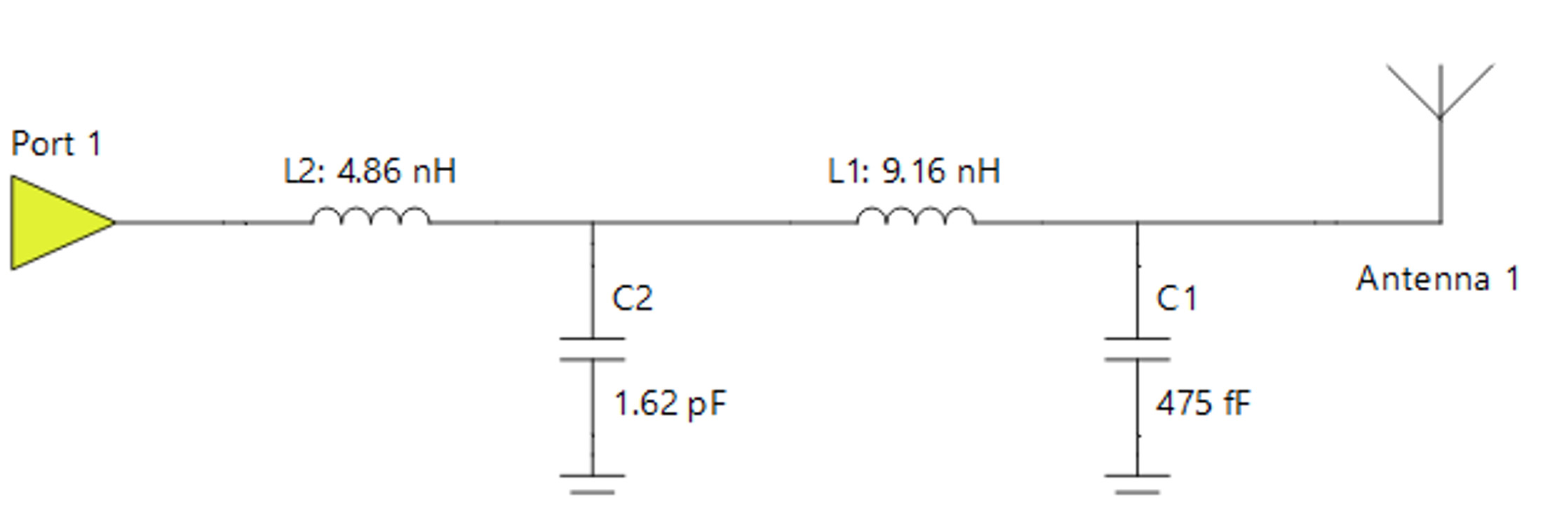
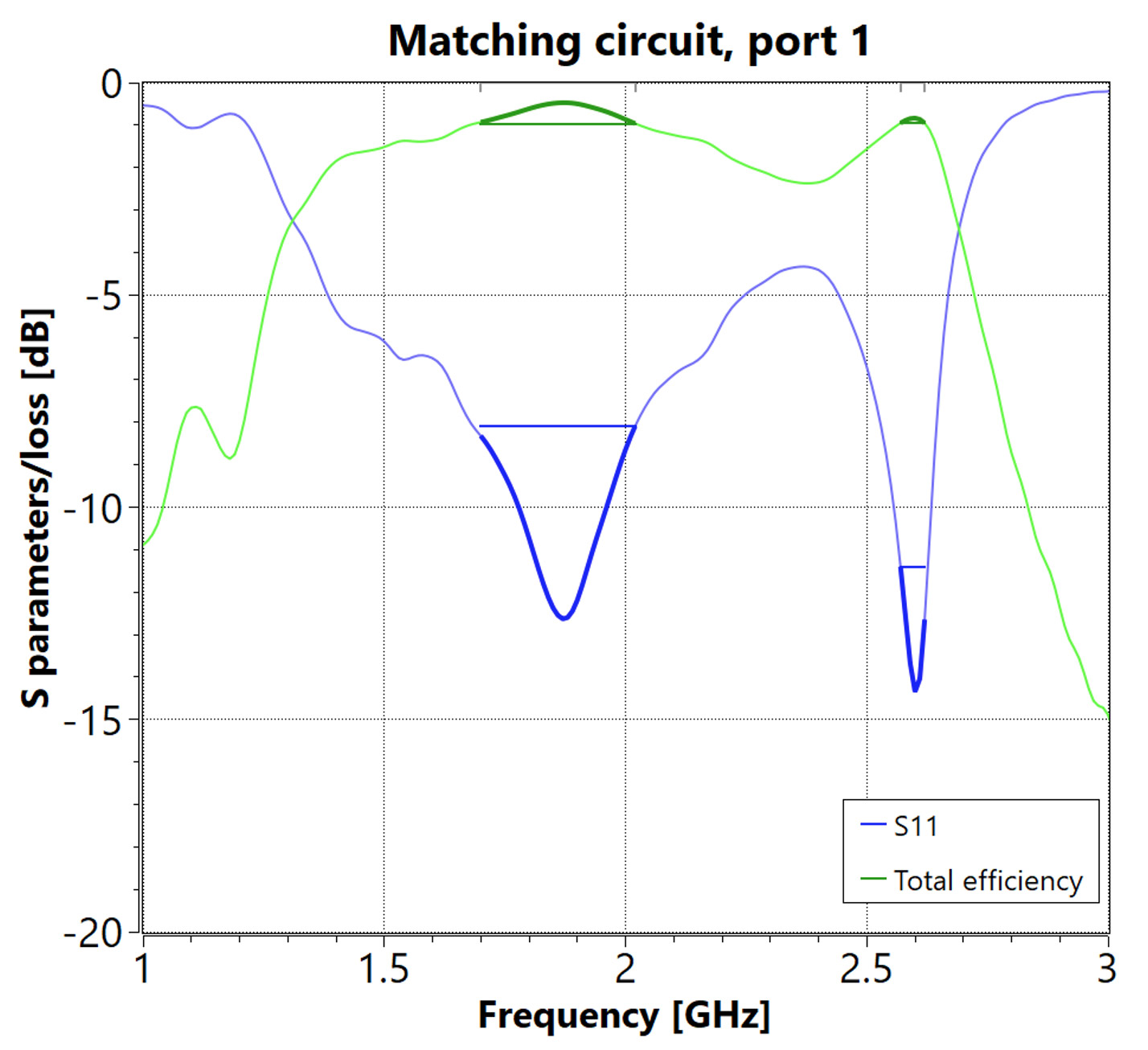
And this is the frequency response result
So in all, a manual tinkering worth of more than 4 hours in a traditional RF circuit simulation and optimization tool was reduced to a design task taking less than 40 seconds in a Optenni Lab.
But wait – when we write “the best result”, exactly what do we mean?
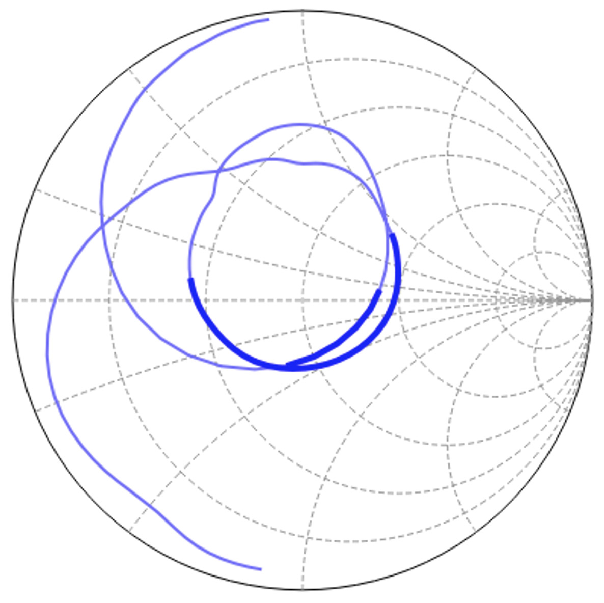
To cut the long story short, the best result (in this case) is the result with the best worst-case performance of the efficiencies over the two frequency bands. So the S11 of the matching circuit is just a starting point, and it is the efficiency that counts. Note, however, that the S11 has the valleys / notches at the frequencies where the efficiency peaks. This is reflected also in the Smith chart with S11 arches that loop around the center of the Smith chart as closely as possible at the bands of interest as the frequency varies. If the S11 would go through the Smith chart center, the matching would likely be excellent, but only in that single spot frequency, and far off in the other frequencies.
Conclusion
This was maybe one of the most simple use cases of Optenni Lab but it goes a long way to illustrate one of the prime ways Optenni Lab accelerates the design flow by
- focusing on the most important figure of merit in making well-radiating antennas, the optimization total efficiency, and
- by synthesizing circuits automatically instead of forcing the user to manually tinker with horde of circuit topologies.
Of course Optenni Lab offers so much more even for a single-port matching, with built in support for library components, their statistical, sensitivity and tolerance analyses, versatile user interface for result management and post processing etc. And things get even more exciting with multiport matching. We will cover the ways Optenni Lab can accelerate your design work in later blog articles.
info (at) optenni.com