Exploring Antennas With Optenni Lab
Introduction
With the blog article of September 2023, we touched the main design philosophy of Optenni Lab, where the user may Explore the antenna, Accelerate the design of antenna matching, and Maximise the impact of matching.
In this blog article, let me focus on the first aspect of this philosophy, Explore.
Before matching circuits are synthesized and time is spent to gain adequate performance, it is very beneficial to get an overview of the theoretical limits of the antenna’s radiator. If the radiator has very little chance of surviving the communication task at hand, it is better to go back to the drawing board and try to redesign the radiator. After all, if a failure is to happen in engineering, it always pays off to fail fast and in early stages of the design, and then move on.
Optenni Lab Preassessment tools
There are three main preassessment tools in Optenni Lab: Bandwidth potential, electromagnetic isolation and total scan pattern.
Electromagnetic isolation can reveal that the isolation between two antenna ports is, in fact, caused by poor matching. If we take away the effect of poor matching, it may become evident that the two antenna ports are quite strongly coupled. This can become a problem for antenna systems with many radiators.
Total scan pattern is an important feature in assessing the ability of array antennas to direct radiation over the solid angle enclosing the array.
Preassessment Workhorse – The Bandwidth Potential
Bandwidth potential is likely the most frequently used preassessment tool in Optenni Lab. It gives a quick overview on the following: What is the width of the frequency band at each of the frequencies available in the antenna impedance data (Touchstone file) if we wish to reach a certain matching level (using an ideal two-port matching circuit).
A typical bandwidth potential graph is given in Figure 1 below. It shows that the antenna in question will be difficult to match to -10 dB return loss level at frequencies below 1.3 GHz. At approximately 1.8 GHz a massive bandwidth of 700 MHz is easily achievable. Again, at around 3.6 GHz a broadband matching of more than 100 MHz (twice the indicated potential of 50 MHz for a two-port matching) will likely be hard. And finally, around 4.4 GHz, a 700 MHz bandwidth will again be a simple task.
It is very typical that the bandwidth potential tapers out at both edges of the frequency spectrum, as the number of frequency points runs out (the closer we get to the start or end of the frequency data, the more narrow the bandwidth potential becomes out of necessity). Also at low frequencies, antennas tend to be short in terms of wavelength, and thus the ability of the antenna to radiate is quite limited, dropping the bandwidth potential further.
With single port antennas, the usage of bandwidth potential computation is very straightforward. Just go to the Assessment menu and choose Bandwidth Potential, set the matching level, and off you go, as in Figure 1.
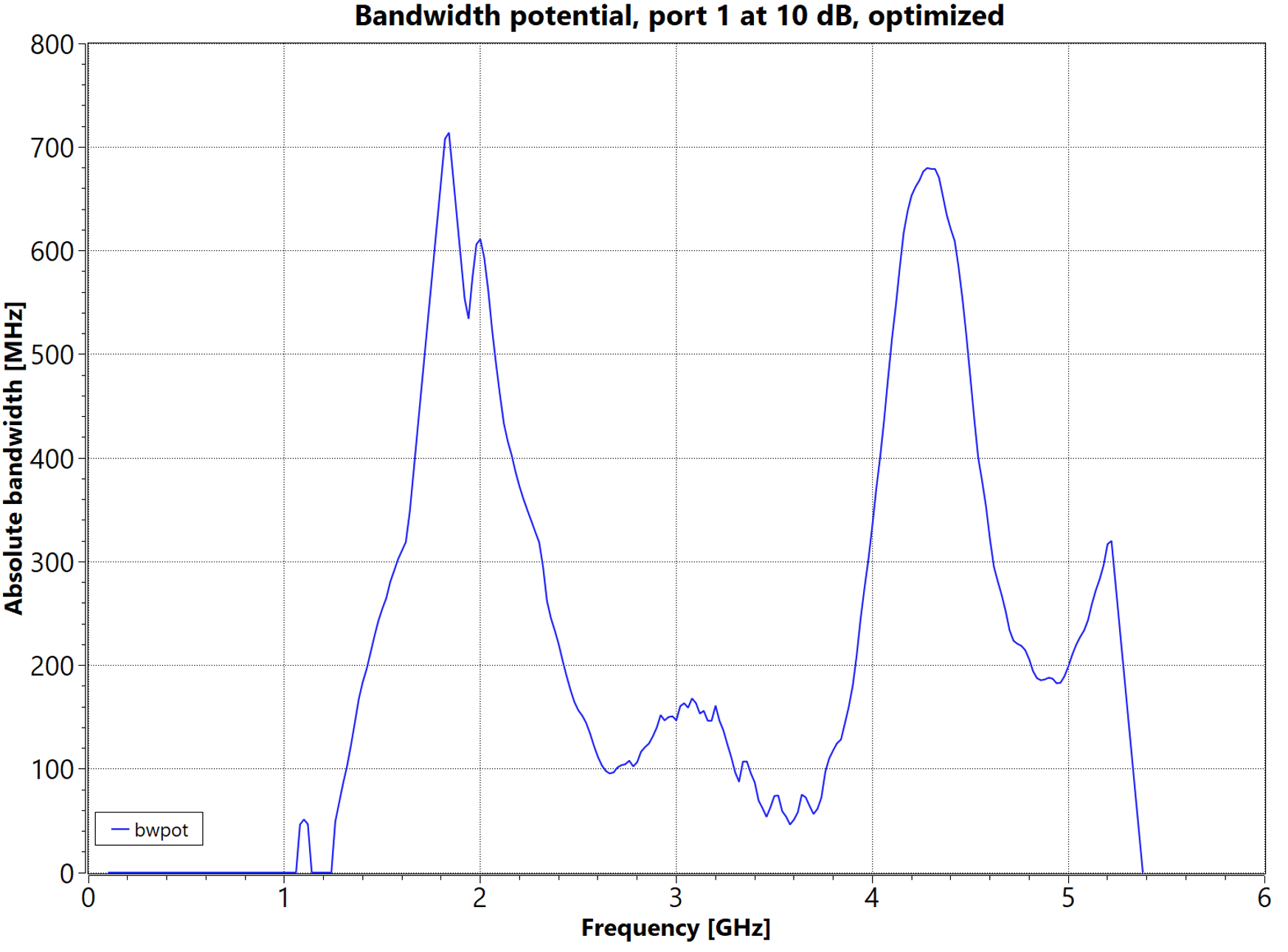
Figure 1: Bandwidth potential reveals the performance of the bare antenna in terms of bandwidths
The Bandwidth Potential of Multiport Antennas
When the antenna is a multiport antenna, for example an aperture tuned two-port structure, things get a lot more interesting!
Consider the basic building blocks of an aperture tuned antenna with a feeding port 1 and tuning port 2 as shown in Figure 2. Green portion marks the meal strips of the radiator, and orange portions are the conducting ground plane. Tuning port 2 has a switch element with various load impedances (inductors or capacitors), that can be dynamically connected to the second port 2.
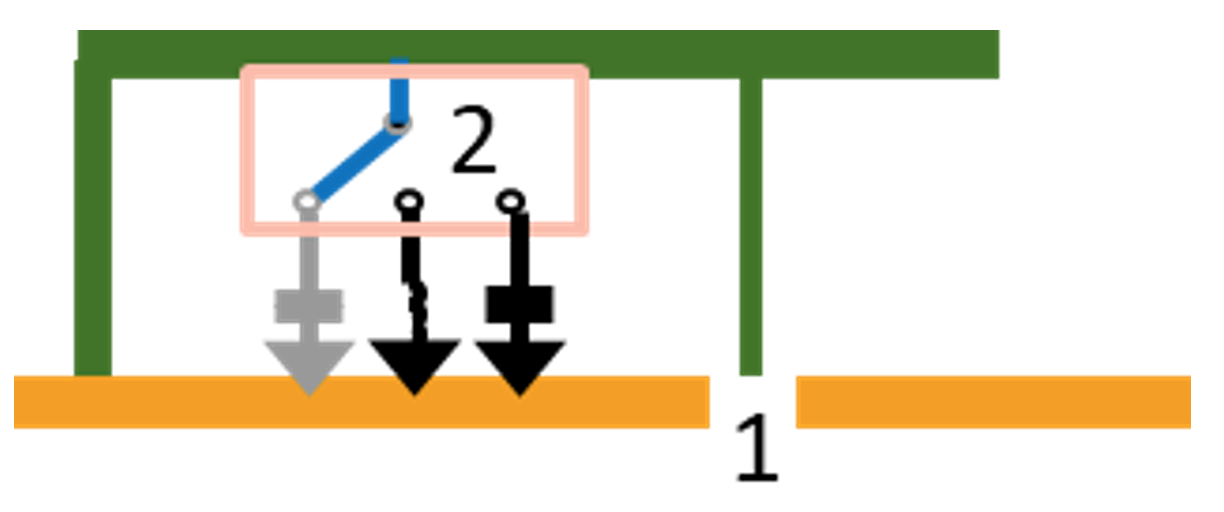
Figure 2: Basic building blocks of an aperture tuned antenna
Let’s also assume that the antenna is to operate at three distinct frequency bands, and let’s call them
- “low band” at 800 – 900 MHz,
- “mid band” at 1700 – 1800 MHz, and
- and “high band” at 2500 – 2700 MHz,
so that for each of the bands, the switch is at one of its throw positions.
Now the basic design challenge is: What kind of static matching circuit is the best for port 1, and what the three tuning components should be in port 2?
But before we give this task for Optenni Lab to be solved, we can look into the bandwidth potential of the antenna so that we try different tuning port loads at port 2, and see how things look like from port 1.
In version 6.0 of Optenni Lab, studying tuning port loads together with bandwidth potential is really quite simple. In the past, the user had to export one-port S-parameter file and open it in an “auxiliary project” to generate the bandwidth potential graph. Not anymore! As shown in Figure 3, simply first terminate the port 2 with a load you wish to study (say, a 1 nH inductor).
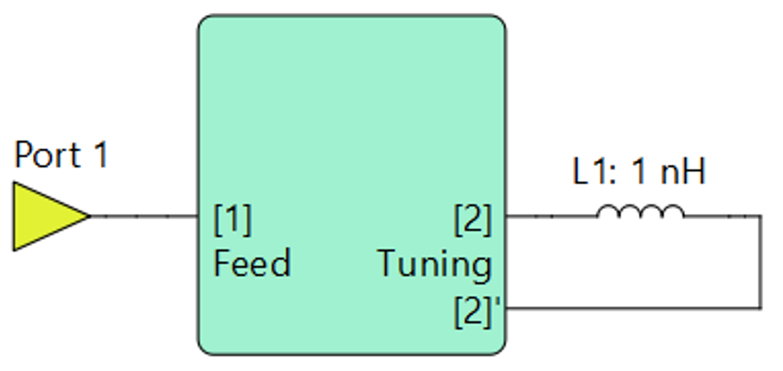
Figure 3: Aperture tuned antenna subjected to 1 nH tuning port load
Then, choose Additional plots… from the plot selection panel,
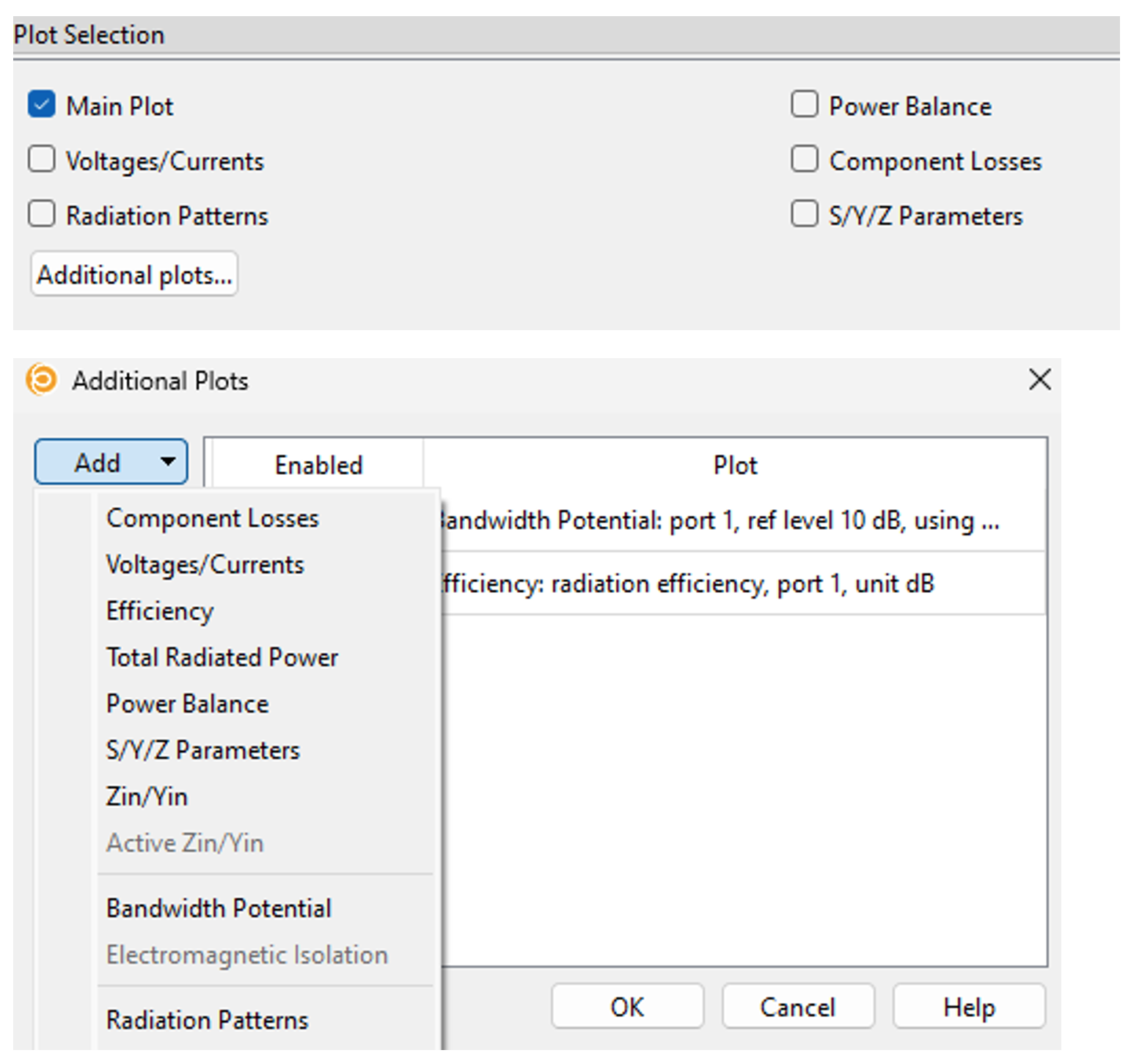
Figure 4: Bandwidth potential is now accessible through Additional Plots
Add Bandwidth potential and Radiation efficiency as plot types.
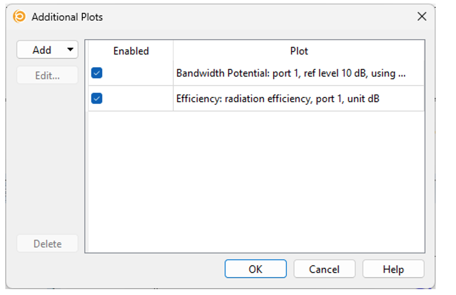
Figure 5: Bandwidth potential and efficiency can be turned on or off
Finally, set the bandwidth potential parameters (matching level and symmetry).
At the same time, it is also beneficial to study the radiation efficiency of the radiator. As the tuner port load changes the currents of the radiator, the tuner port changes also the radiation efficiency. This aspect is easily overlooked when designing tunable antennas.
Figures 6 and 7 show typical results for the resulting bandwidth potential and for radiation efficiency, respectively.
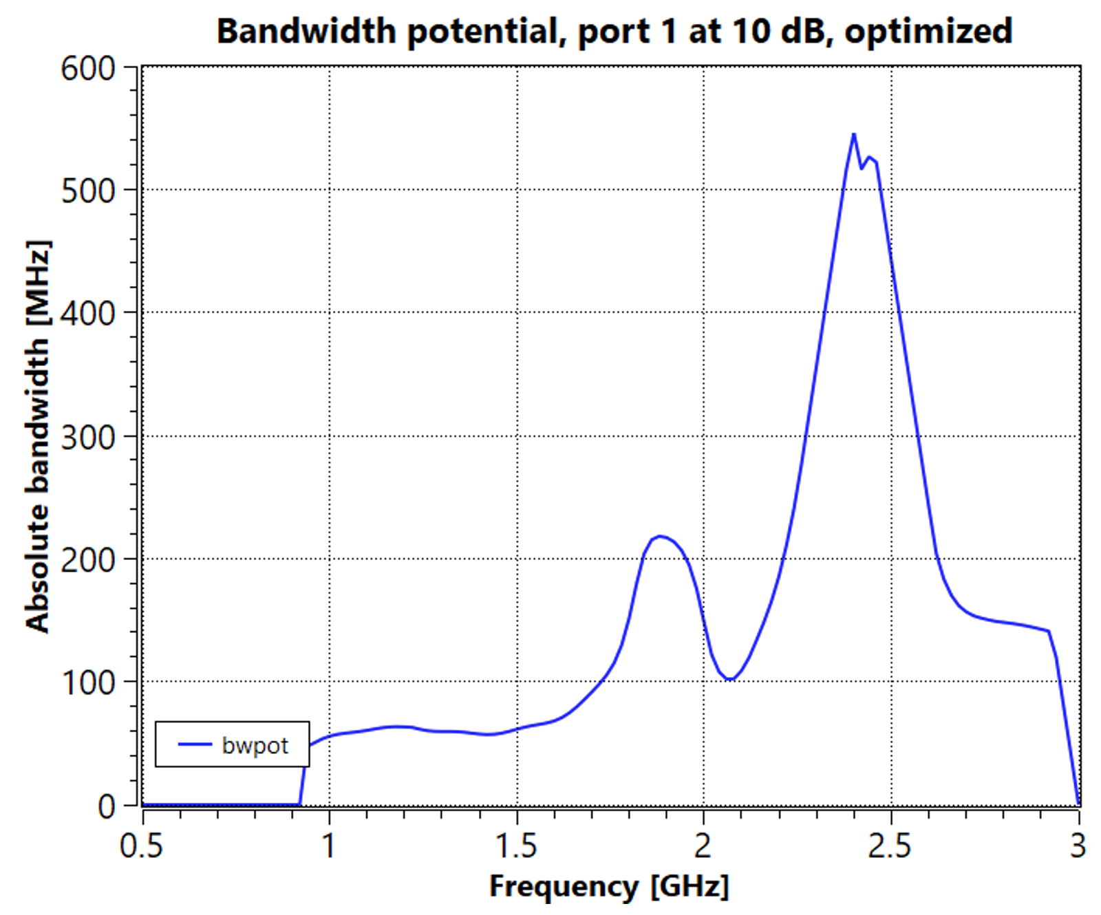
Figure 6: Bandwidth potential with a 1 nH load in the tuning port 2
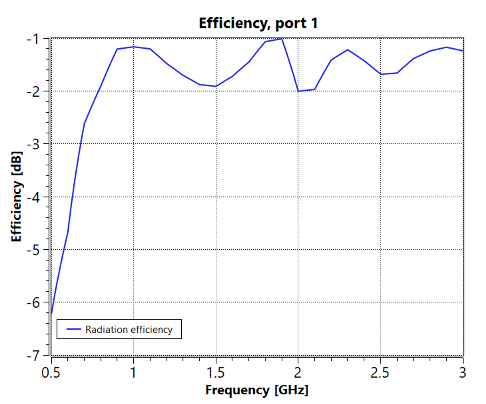
Figure 7: Radiation efficiency with a 1 nH load in the tuning port 2
As an additional plot, bandwidth potential computation is a game changing feature in Optenni Lab 6.0! It makes the generation of bandwidth potential chart (where several bandwidth potential curves are stacked) almost trivial. Simply tune the load at port 2 to get a selection of bandwidth potentials related to various inductance loads. You may then go also through some capacitor values, and short and open circuit options in port 2. Then, push all these results to a User Plot, and you easily get the following kind of chart:
At the same time, it is very easy to generate the following radiation efficiency chart, almost as a by-product.
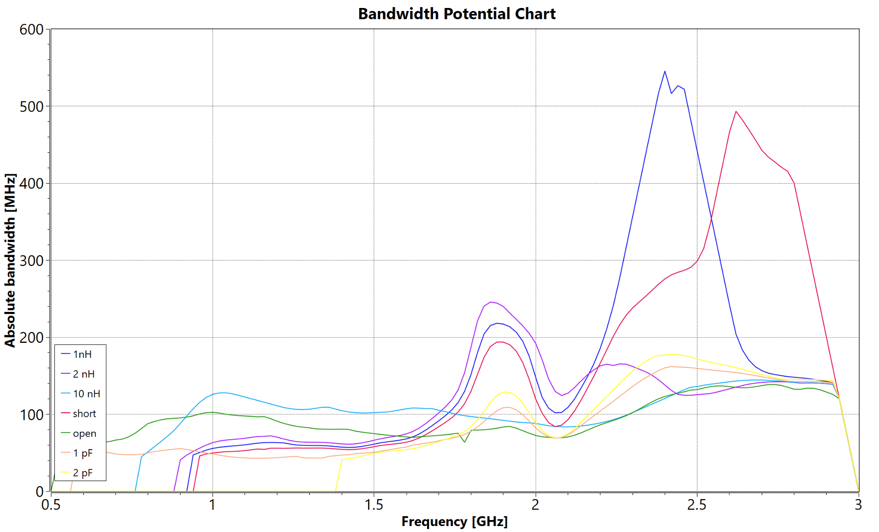
Figure 8: Bandwidth potential chart
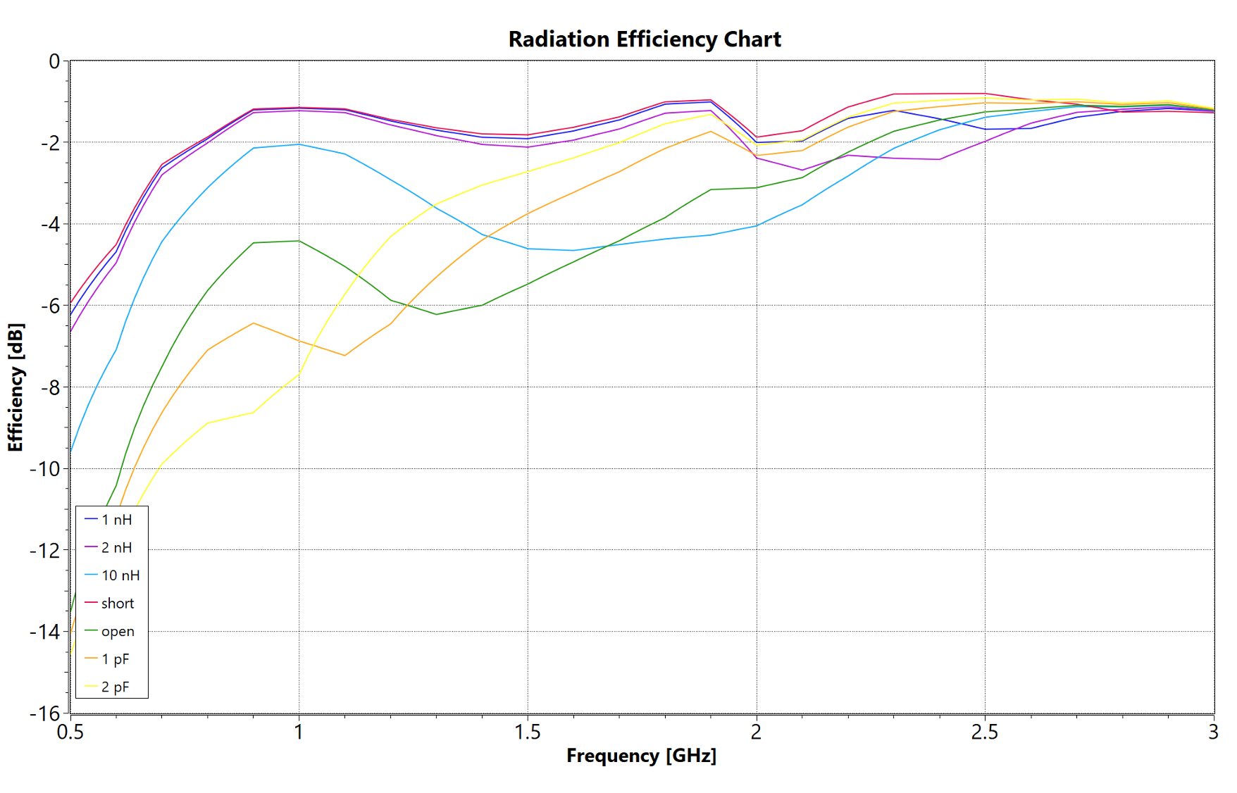
Figure 9: Radiation efficiency chart
Interpreting Bandwidth Potential and Radiation Efficiency Charts
Now let’s see what these two charts reveal for us.
For high band at 2500 – 2700 MHz, the choice of tuning component is clear: The best bandwidth potential is achieved with a short, and as the radiation efficiency is more or less independent of the tuner loading (as the curves are stacked on top of each other around 2500 – 2700 MHz), we can safely assume that the switch should couple to a short when the antenna is operating in the high band.
In the middle band at 1700 – 1800 MHz, both the bandwidth potential and radiation efficiency are at their highest values when there is a small, 1 – 2 nH inductor in the tuning port. Thus, we can let Optenni Lab optimize the inductor value, but there appears to be no need to consider also a capacitor in the tuning port at the middle band.
For the low band at 800 – 900 MHz, the radiation efficiency is again quite good with small inductors, but the bandwidth potential is really poor (more or less zero) for these loads. However, there seems to be a compromise based on a large inductor (10 nH) value, which implies a large impedance. Such a large impedance can also be a small capacitance. Thus, it is likely best that this tuning component is left for Optenni Lab to choose, based on the versatile Generic Reactance component.
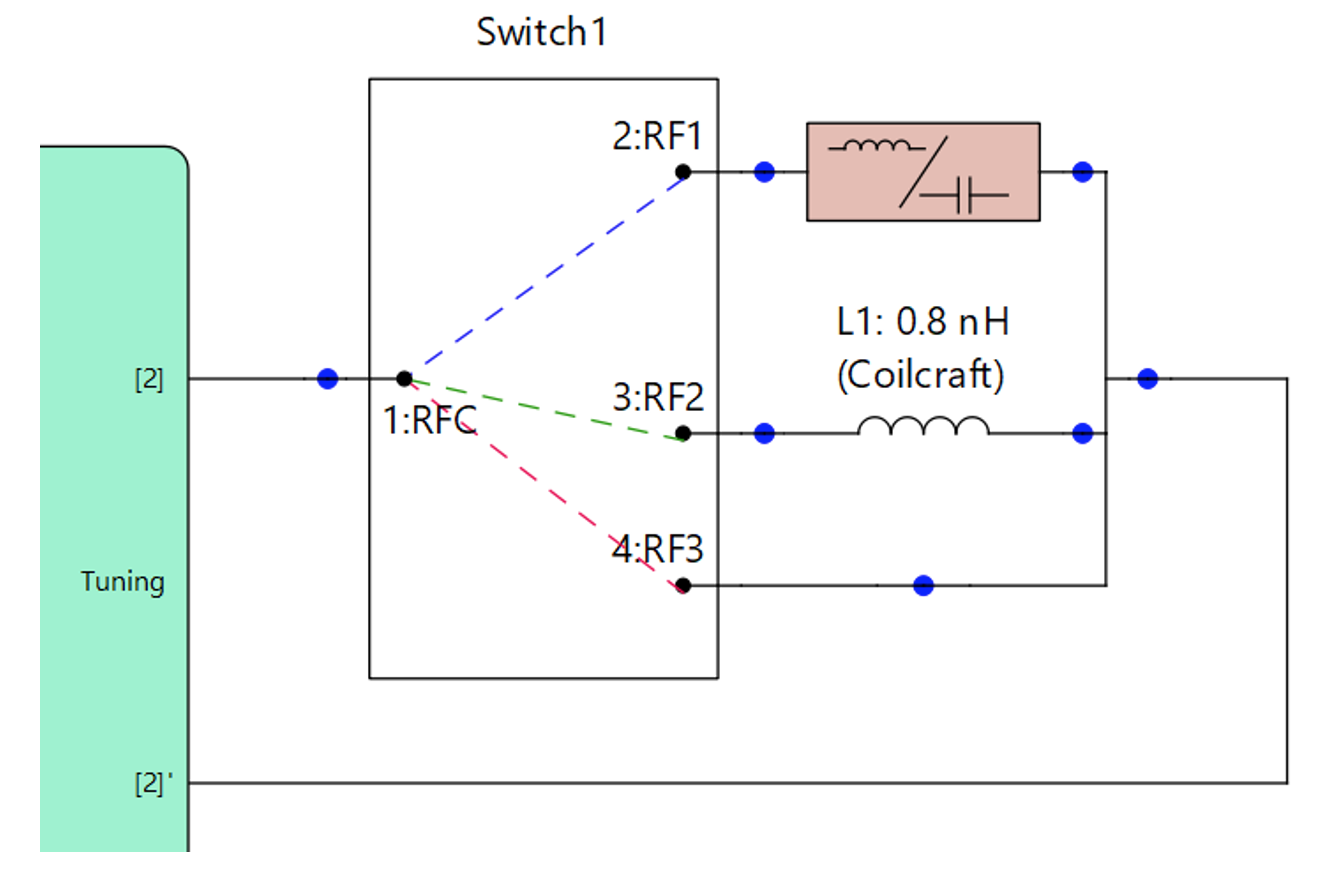
Figure 10: Tuner optimization setup (RF1 – low band throw port, RF2 – mid band throw port, RF3 – high band throw port)
Benefits of this approach are clear:
- For the high band, nothing needs to be synthesized or even optimized as there is simply a short in this port,
- For the middle band, we just need to optimize for inductors, not for capacitors at all.
Ability to omit these two synthesis steps saves time considerably.
Conclusion
Taking a critical look into the radiator before any matching is attempted is usually very beneficial, especially for tunable antennas where the synthesis times can be long. With the bandwidth potential and radiation efficiency plots, the secrets of a tunable radiator become a lot more visible even when the tuning port load is varied.
If both bandwidth potential and radiation efficiency are low for any tuning port load and at any one of the frequency bands, redesign of the radiator of the tunable antenna should be considered. On the other hand, if any of the tuning components seems to indicate a good performance in both bandwidth potential and radiation efficiency, we can likely choose that component as a starting point for synthesis, and sometimes even set its value (especially for short or open circuits) without doing any synthesis or optimization. This speeds up the synthesis task considerably and gives the antenna designer a firm handle on the potential performance of the tuned antenna radiator, even before any matching is attempted.
info (at) optenni.com