Matching with Optenni Lab When the Environment Loads the Antenna
Introduction
As discussed in previous Optenni blogs already, modern day antenna designers face major challenges with limited antenna sizes, multiband & wideband operation and good radiation efficiency requirements. But this is not all. In reality, no antenna is suspended in static, immutable free space. Real antennas are used in variable environments, and this alters the ways electromagnetic waves are sent and received by the antenna. For example, mobile phone antennas should perform adequately when the phone is on the table, operated next to user’s head or when the phone is left in a purse. Laptops might have their lid open or closed. Even the smallest of variations in the placement of a hearing aid changes the antenna performance of the Bluetooth connection of the device.
In practice, different operating environments cause variations in both port impedance and radiation pattern of the antenna. In antenna parlance, the environment is said to “load” the antenna.
It is evident that the variations in impedance and radiation pattern pose yet another degree of difficulty to the antenna designer. For what impedance or loading condition should the matching be attempted? How to study the impact of loading to the antenna performance? These are the topics of this blog posting.
Example Structure
For the sake of discussion, let’s study a planar inverted F antenna (PIFA) suspended over a ground plane (blue portions) placed vertically, fed with a port marked red, and loaded by a dielectric cover shown in yellow. In Figure 1 a), the cover is directly over and in contact with the radiator of the antenna. In Figure 1 b) the cover is slightly separated, and in Figure 1 c) the antenna is placed in free space. Clearly, such scenarios are realistic in the various operating environments of the antenna.
How would you design one matching circuit that covers all these three cases in the best possible way?
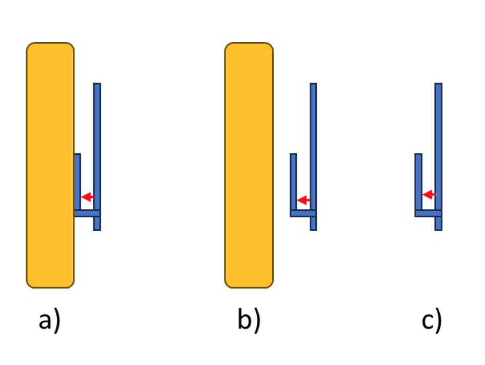
Figure 1 – three operating environments of the antenna
The Optenni Lab Approach
Optenni Lab solves this design challenge with a concept called “Impedance Configurations”. Each impedance file (say, one port Touchstone S-parameter file) and, if needed, efficiency data or radiation pattern data can be separately imported into Optenni Lab as one Impedance Configuration. Here we deal with just three single port Touchstone files, but multiport antennas, radiation patterns and efficiency files are studied with similar ease.
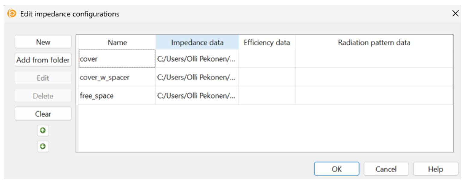
Figure 2: Optenni Lab makes operating with several impedance datasets a breeze – just add them as Impedance Configurations
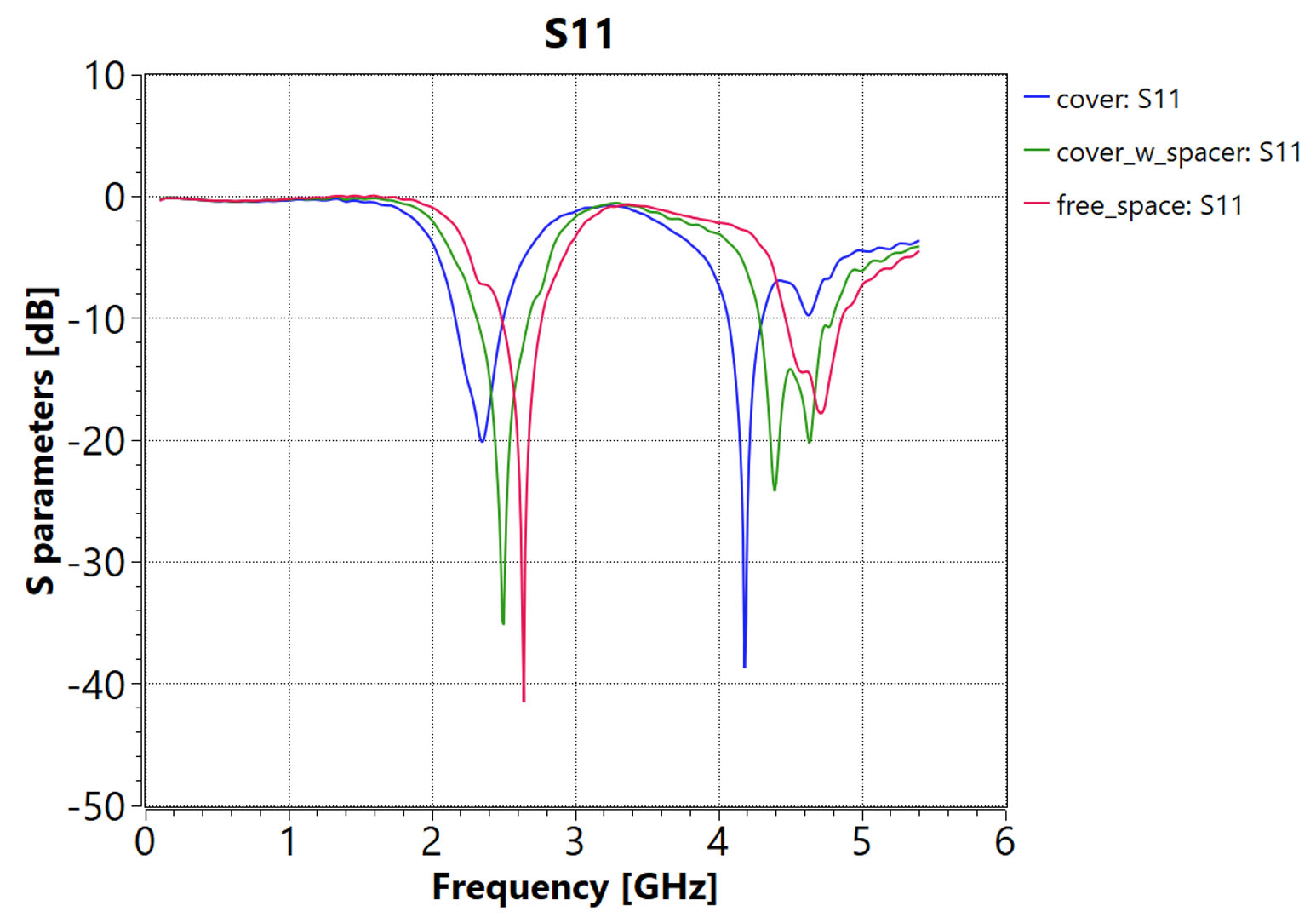
Figure 3: The three Impedance Configurations as starting data for the matching synthesis
Looking at Figure 3, it is evident that the antenna’s self-matched frequency (denoted with a notch in the S11 curve) wanders when the antenna is loaded with the cover. This is easy to understand as the dielectric loading makes the antenna see the surrounding space to comprise material with εr > 1. The free space case has the notch at the highest frequency (at 2.64 GHz), and the most loaded case (cover in contact with the radiator) has the lowest frequency for the notch (at 2.35 GHz).
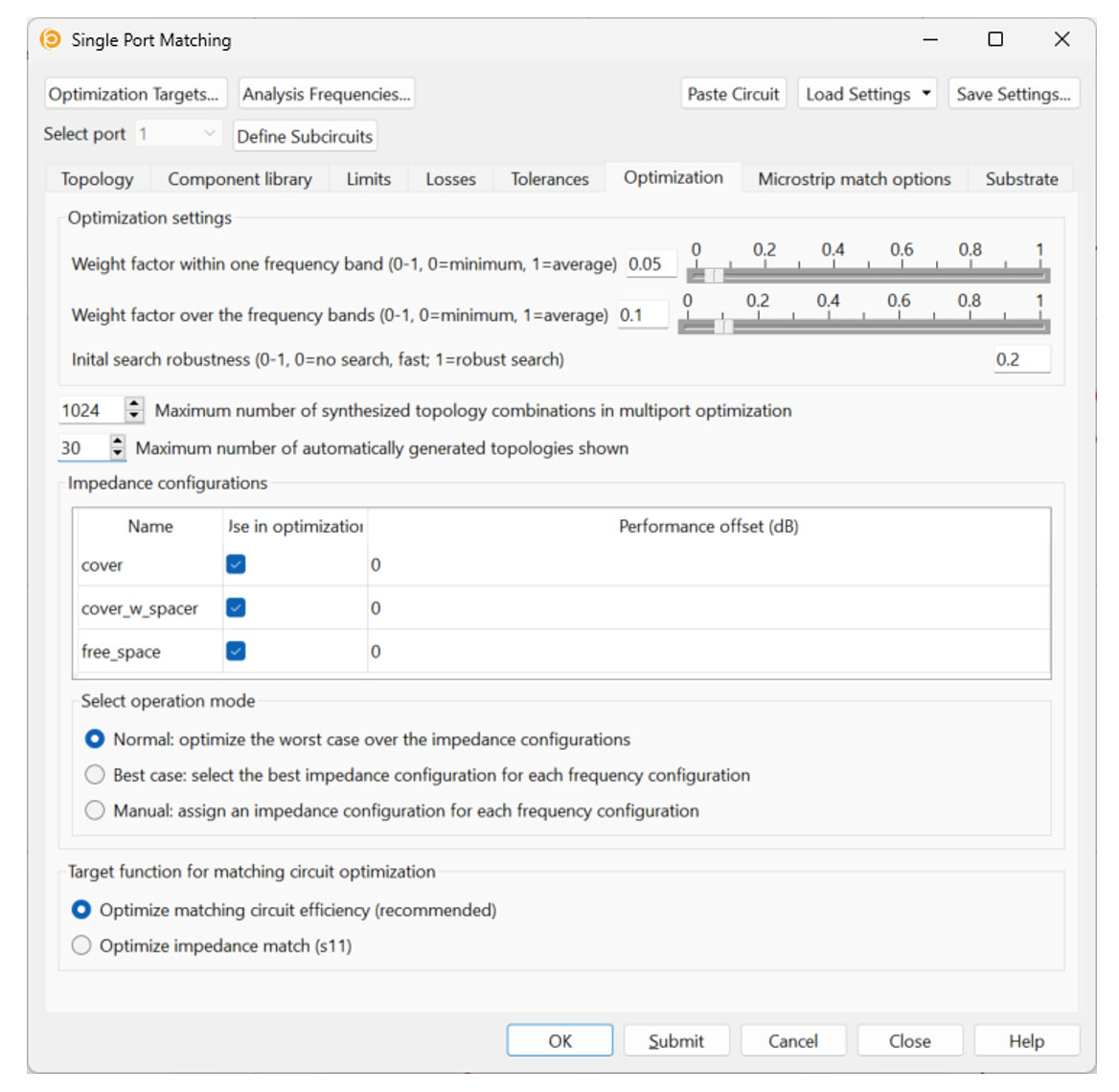
Figure 4: In Optenni Lab version 6.0, Impedance Configurations are managed from the Optimization tab. In this case we wish to optimize the worst-case over the Impedance Configurations, but other options exist, too. It is also possible to set a performance offset if some Configurations are deemed more important than others
With these settings, operating Optenni Lab with three sets of impedance data is exactly as simple as operating it with a single one. Seeking a good matching in WLAN (2.4 – 2.483 GHz) and 3GPP Band 7 bands (2.5 – 2.69 GHz), a result which satisfies best all the three Impedance Configurations is show in Figures 5 and 6, using library components from Murata and Coilcraft:
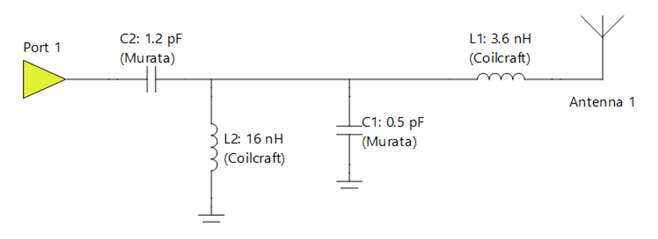
Figure 5: Optimal matching circuit with four components
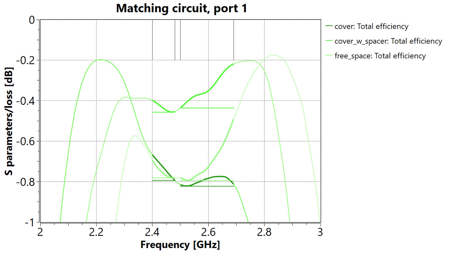
Figure 6: The efficiencies obtained over the bands, and with the three Impedance Configurations. Note that the worst-case level is around -0.8dB
With cost function -0.8dB in the worst-case of the three Impedance Configurations (indicating 0.8dB distance to a perfectly matched case at the two bands of interest, in the worst spot over the bands), the matching satisfied all three configurations very well.
Also a very elegant result with a cost function of -1.1dB is found, comprising only one shunt inductor.
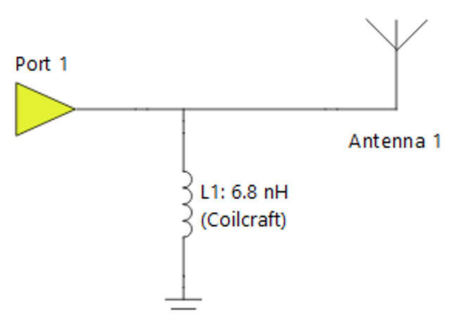
Figure 7: A very elegant solution with a cost function of -1.1dB.
What if Impedance Configurations are not available
Here in Optenni, frankly we are not sure how the design challenge described above is best solved without Optenni Lab’s Impedance Configurations. As one approach, one can speculate that using an “average” representation of the loading of the antenna, we could derive a “best-for-all” matching. In this case it would likely be the “cover which is separated” (see Figure 1b) case.
So lets see how this average loading idea plays out. We first take the separated cover related impedance file as a starting point, and perform the matching over the same bands and component libraries, and get the circuit as in Figure 8.
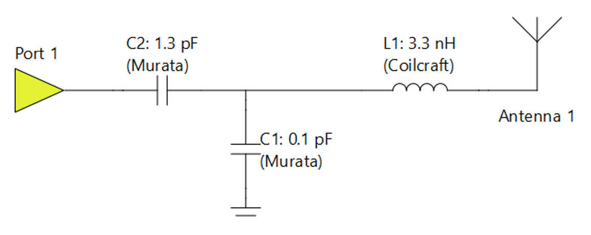
Figure 8: Matching circuit for the cover with separation case alone
As is evident from Figure 9 below, this is a very easy matching task yielding an excellent efficiency/cost function of -0.2dB in the worst-case.
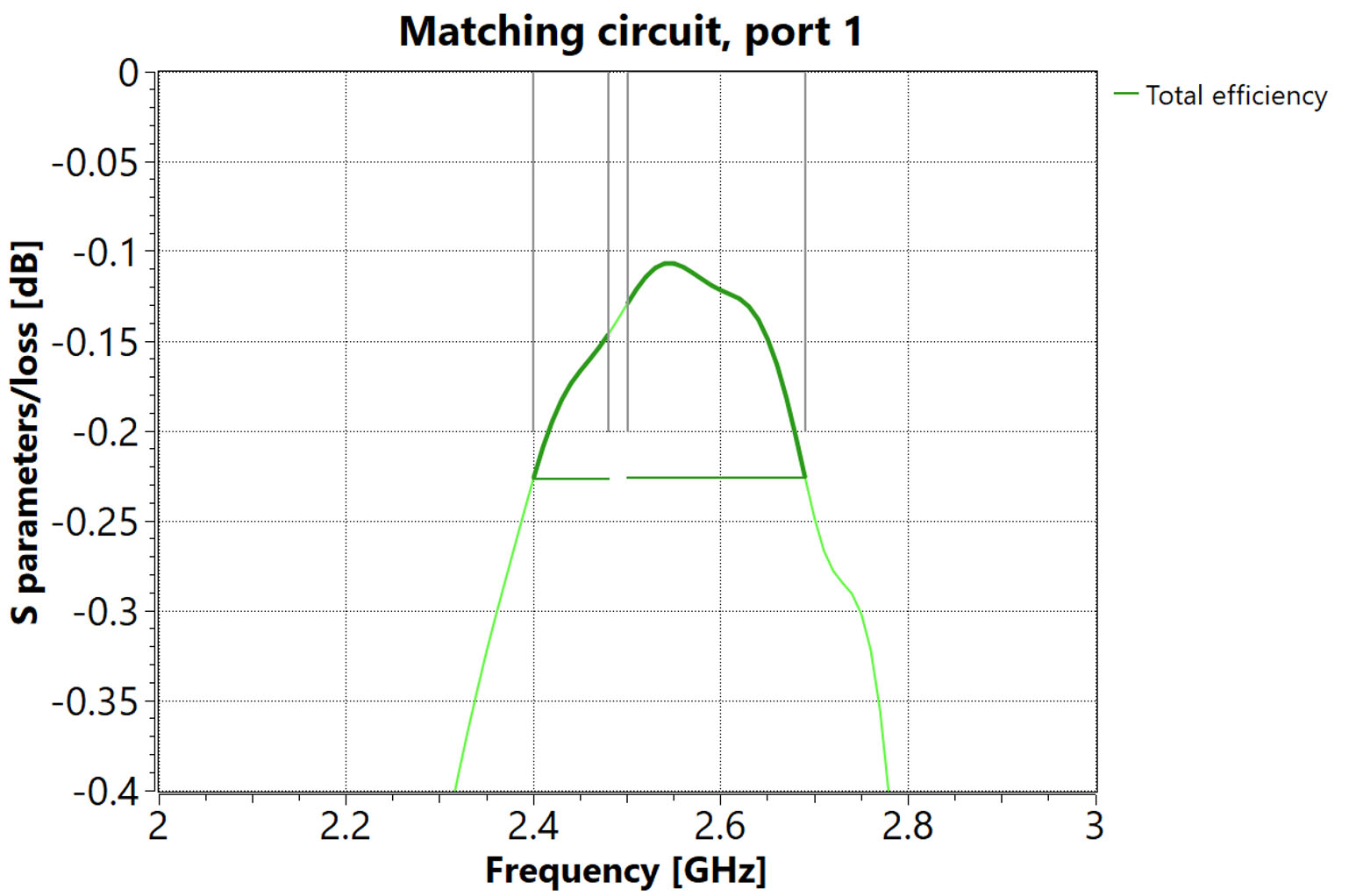
Figure 9: The single matching result is excellent… but how does the circuit perform with other impedance cases?
But how do things play out with the other impedance files? By fixing the circuit of Figure 8 and setting the antenna impedance to the free space case, we obtain a cost function of -0.8dB. By setting the antenna impedance to the case with the cover, the cost function is -1.3dB. Thus, over the three possible antenna loading scenarios, Impedance Configurations are able to find a better worst-case performance (-0.8dB vs -1.3dB) than the trick of using some “average” antenna loading scenario. Also, in a more general sense, it is not even clear what “an average” antenna loading scenario even might be.
Thus, it is evident that Impedance Configurations add value to design challenges where the antenna is subject to various environmental loadings.
Conclusions
Optenni Lab makes operating with several impedance files simultaneously very easy. In real life, an antenna is never completely stationary in a three-dimensional immutable space. Instead, every change in the vicinity of the antenna will change the impedance and radiation of the antenna.
Optenni Lab is the best-in-class tool to study the loading effects of the antenna and to design matching circuits that do not fail in real-life use cases.
PS. For those willing to try out Impedance Configurations directly, the related tutorial is available in Optenni Lab’s Help > Documentation.
info (at) optenni.com