Unveiling the Impact of Ground Currents on Antenna Matching Circuit Optimization
From this article, you will learn about:
- Component modeling: the importance of accurate component models
- How to assess the ground currents and a practical way to evaluate their level for the chosen component candidates
- Design example showcasing:
- a recommended approach for PCB layout modeling
- the impact of ground currents and model accuracy on simulation results
Introduction
In the dynamic world of wireless communication, optimizing antenna performance is paramount. Whether it’s for your Wi-Fi router at home or a satellite communication system in space, antenna matching circuits play a crucial role in ensuring efficient signal transmission. However, achieving optimal performance requires a deep understanding of the intricate interplay between component models and layout considerations, particularly when it comes to the often-overlooked factor of ground currents. In this article, we will show how components exhibiting high ground currents can introduce inaccuracies in the modeling of matching circuits if these ground currents are not accounted for in the simulation.
The World of Component Models:
At first glance, the components used in antenna matching circuits may seem straightforward – inductors and capacitors with just two pins. But beneath this simplicity lies a world of complexity. Internally, these components are represented by two-port networks, and therein lies the challenge. Some component models come with hidden ground currents, which can introduce inaccuracies in our simulations. So, how do we identify these elusive ground currents?
Let’s turn the 2-ports component’s impedance representation into an ABCD matrix:
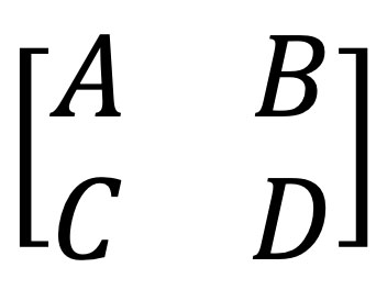
In a real component measurement, any of ABCD terms can represent a complex number. On the other hand, in the case of ideal series connection of a component with no ground reference, the matrix is represented as:
As shown in [1], the parameter is a reliable figure of merit for evaluating coupling to ground. This metric provides valuable insight into how coupling may affect simulation results. For components with low ground currents, the resulting value is negligibly small, whereas for component series with high ground currents, the figure of merit approaches or even significantly exceeds unity.
We used this figure of merit for the components in the Optenni Lab Component Library. Our conclusions from the analysis are the following:
- The majority of manufacturers favour simulation-based models (no ground coupling)
- Some series are measurement-based only for large values
- Some series are fully measurement-based
- Some measurement-based models exhibit problems due to incorrect calibration and de-embedding (non-passivity, unsymmetric behavior or large frequency ripple)
How can I check the component I intend to use exhibits high ground currents?
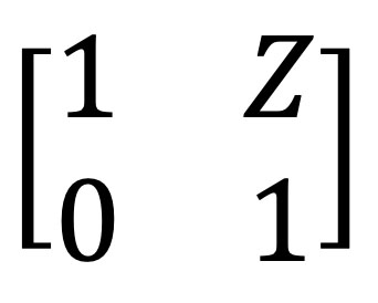
There is no need for complex analysis, such as transforming the component’s S-parameters into an ABCD representation. Instead, you can build a very simple circuit of the component you intend to use and analyse the resulting Smith chart. For example, let’s pick an inductor, place an excitation port on one side, and leave the other side open:
We selected here two simulation results (they are from the analysis we made to study and demonstrate the figure of merit above). One of the results is for an inductor with low reference to ground currents, and the other one is for an inductor with high coupling to ground currents:
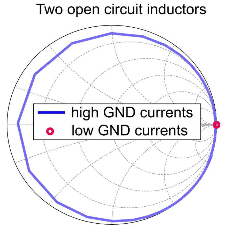
Figure 1. Impedance of two open circuit inductors: (red curve) inductor with low ground currents, (blue curve) inductor with high ground currents.
It is clearly seen from the Smith chart that, in the case of an inductor with low ground currents, all the impedance values are grouped as expected for an ideal open-circuit component (red curve in Figure 1). In contrast, when there is a high level of ground coupling, the curves wrap around the Smith chart, similar to a transmission-line behavior (blue curve in Figure 1). This clearly indicates that the elements cannot be considered ideal lumped components but exhibit a noticeable level of coupling to ground currents.
The Ground Connection Conundrum:
To understand why ground currents matter, let’s delve into the connection between layout and circuit models. Using a two-port S parameter block, we can represent an arbitrary antenna system combined with a component model (Figure 2). Port 1 corresponds to the antenna feed, while Port 2 serves as a component port for a matching component. This representation allows simulation of any single-port antenna system, for example, an aperture-tunable antenna, and is also valid when the component port is connected in series or in parallel with the feeding port:
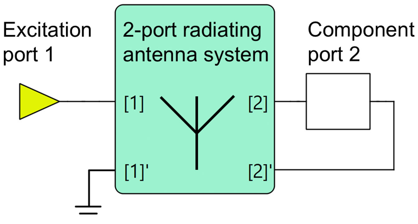
Figure 2. Two-port S parameter block with a matching component model.
In fact, the second port of any component in the circuit analysis requires grounding. In case if physical ground connection is lacking, in the circuit analysis the second node is still grounded artificially, so that the equivalent circuit may be represented as follows:
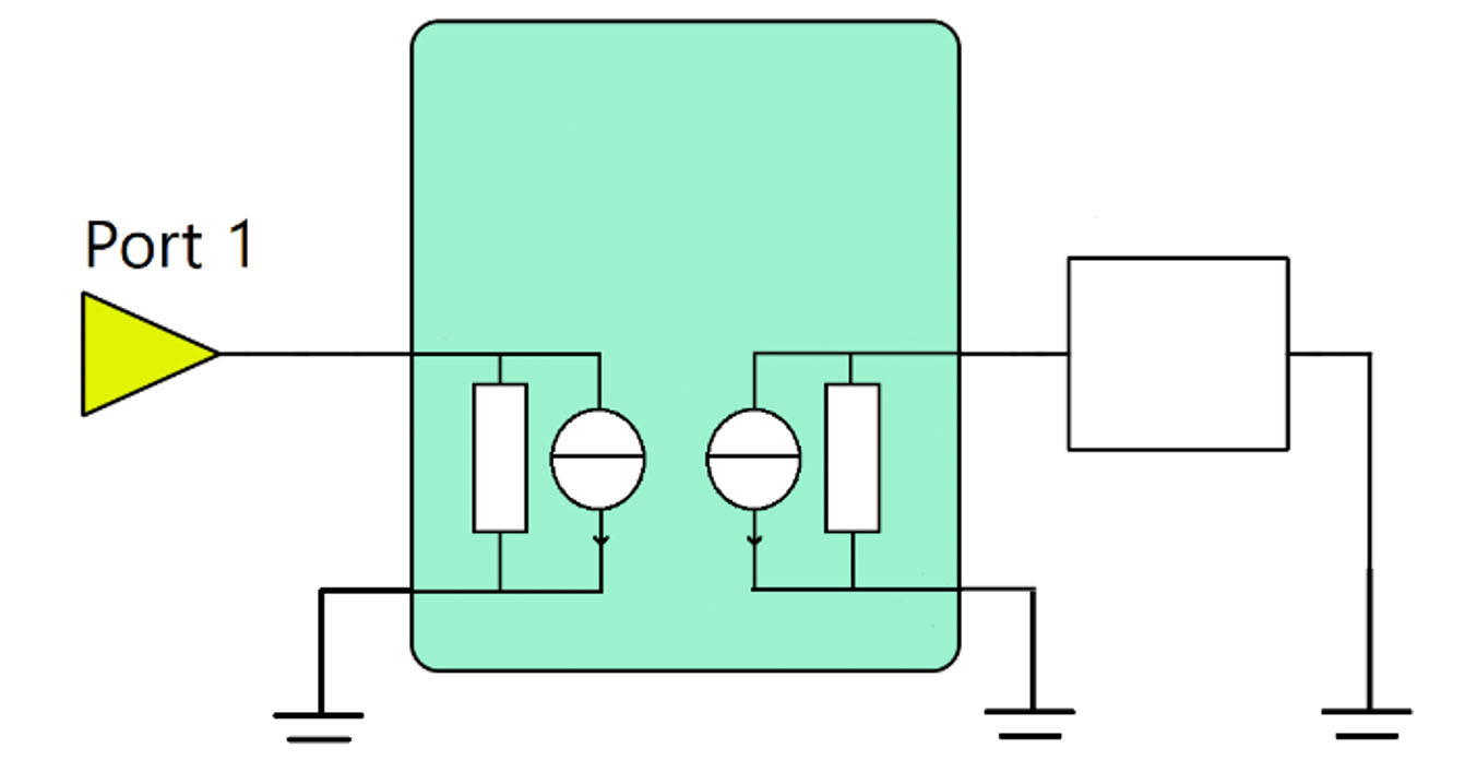
Figure 3. Equivalent circuit for the model with grounding.
Sounds simple, right? Not quite. If there are ground currents lurking within our components, our circuit equations may not tell the whole story. Namely, let’s apply matching, where we explicitly add a circuit with strong coupling to the ground. We will use an inductor as our main matching component, and we can imitate the condition of strong coupling to the ground by adding a component (capacitor) in parallel:
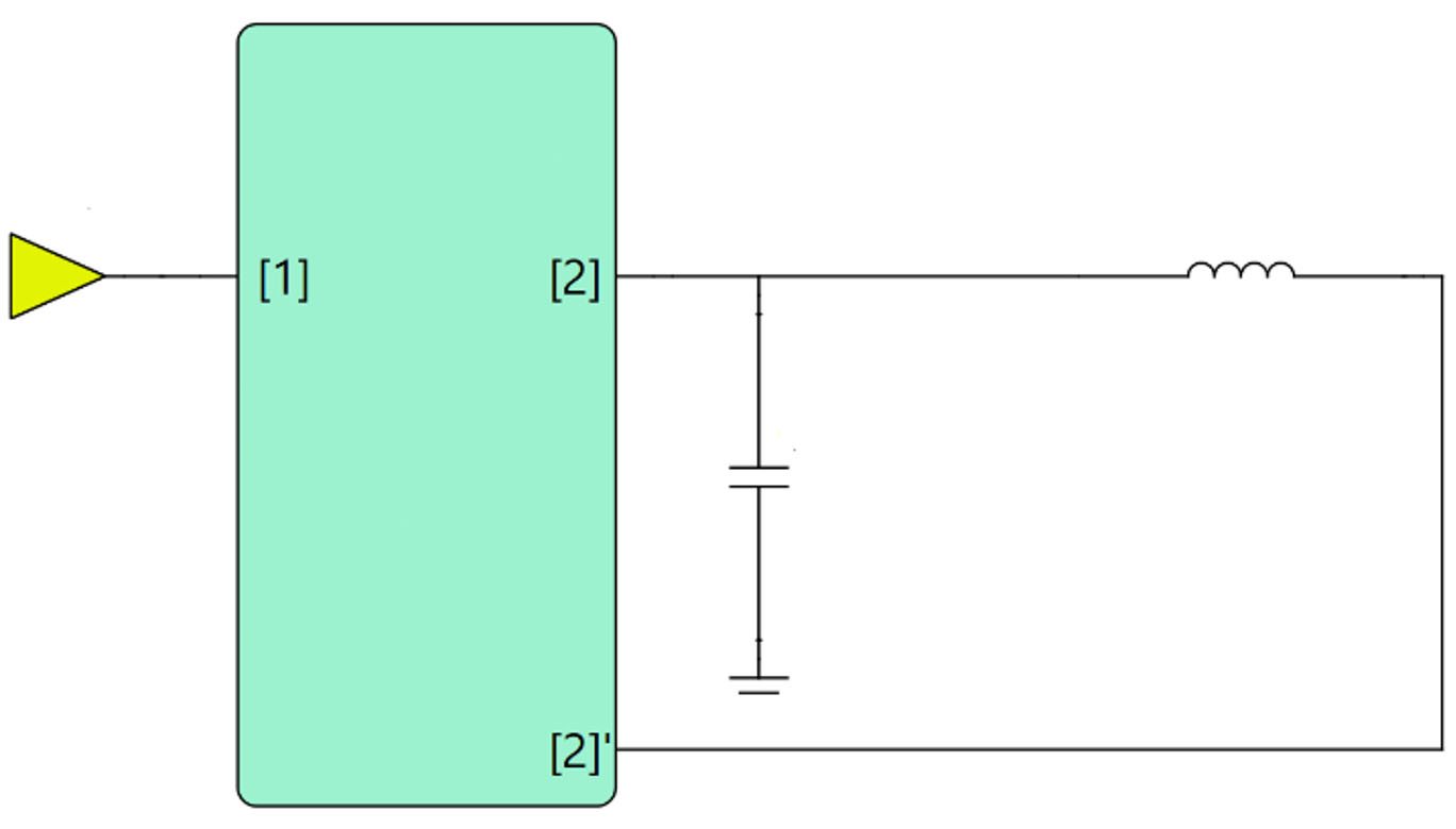
Figure 4. Circuit model with an inductor as the matching component.
However, since we are using the equivalent circuit model shown in Figure 3, adding a ground connection at node [2’] now results in an incorrect parallel resonator (see Figure 5).
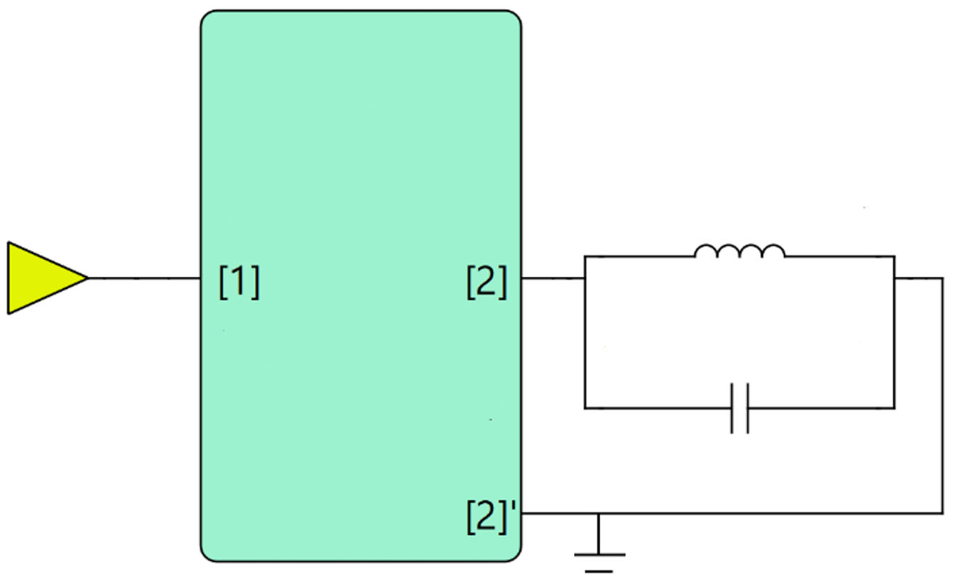
Figure 5. Circuit model with a ground connection at node [2]’ resulting as a false parallel resonator.
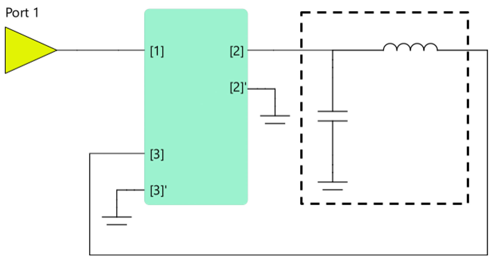
Figure 6. Circuit model with a correctly connected matching component between ports [2] and [3].
Navigating Layout Modeling:
Now, let’s talk about a practical example. Picture your antenna’s layout – a meticulously designed circuit board with matching components strategically placed. We use here a simple prototype of PIFA model with pre-defined matching layout:
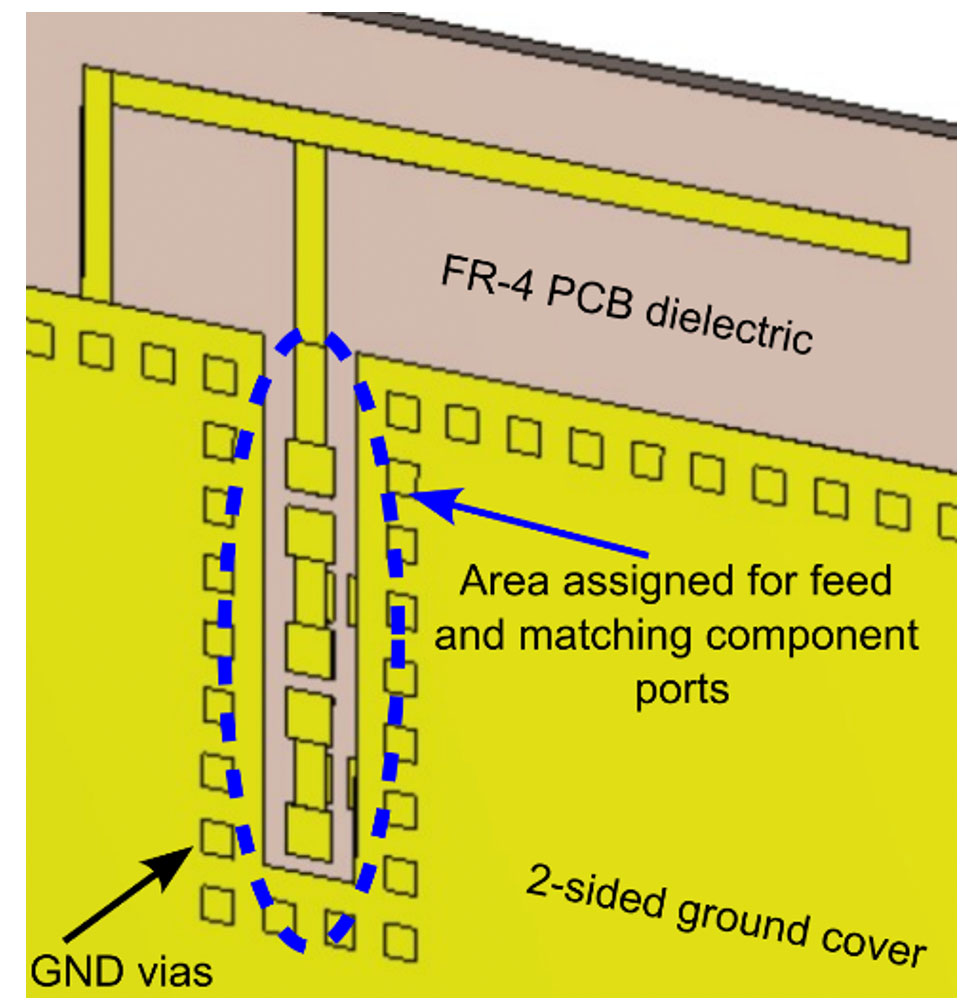
Figure 7. Simulation model including the PIFA antenna and PCB layout for the matching circuit.
When it comes to simulating this layout, we have several options. The first, simpler method applies a single port for each component without explicit reference to the RF ground:
Figure 8. Layout model with no RF ground connection.
Another approach involves using electromagnetic (EM) simulation, where ports refer explicitly to the RF ground. I.e. we have now two ports, and the second node of each port is connected to the bottom ground:
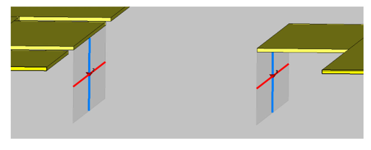
Figure 9. Layout model with ports referring explicitly to the RF ground.
This way we can set the matching component between the nodes of two different component ports and do reference to ground coupling current. So, here’s the kicker:

ignoring ground currents
in our components can
lead us down a perilous
path of inaccurate
simulations.
Numerical Experiments:
To illustrate the importance of considering ground currents, let’s dive into some numerical experiments applying matching components. We’ll compare two modeling methods: one that ignores ground currents and another one that acknowledges them. In the first case, the component is inserted in the component port. In case if the circuit representation does not show the second node of the antenna circuit block, this second component node should be grounded:
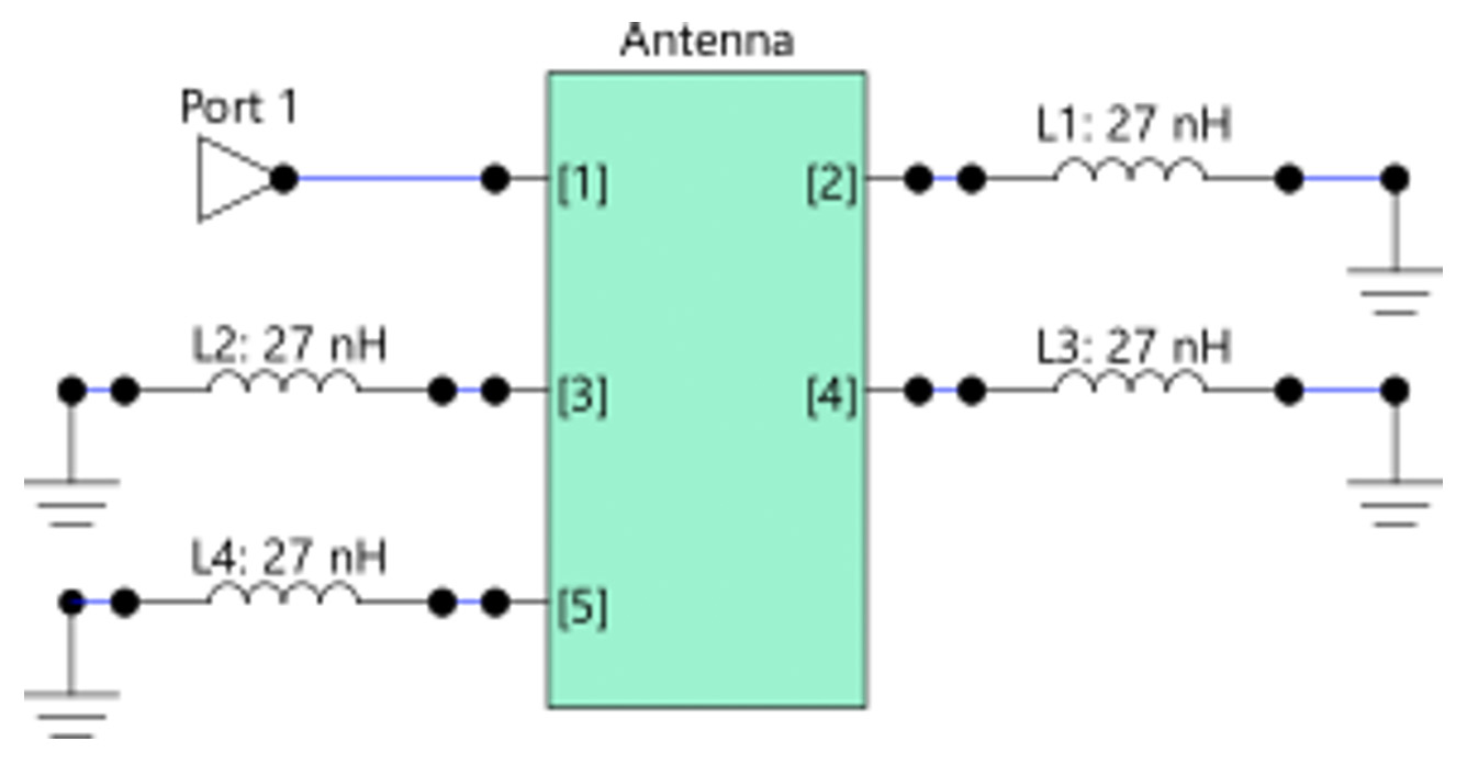
Figure 10. Matching circuit model ignoring the component ground currents (5-port model).
For the second approach we have to connect every component between the corresponding nodes of two ports.
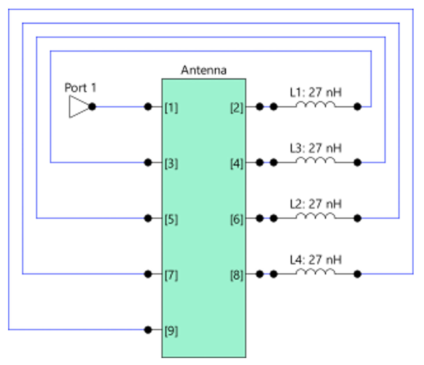
Figure 11. Matching circuit model including the component ground currents (9-port model).
Brace yourself for some surprising results! Let’s see what happens in the case of components with low ground currents applied.
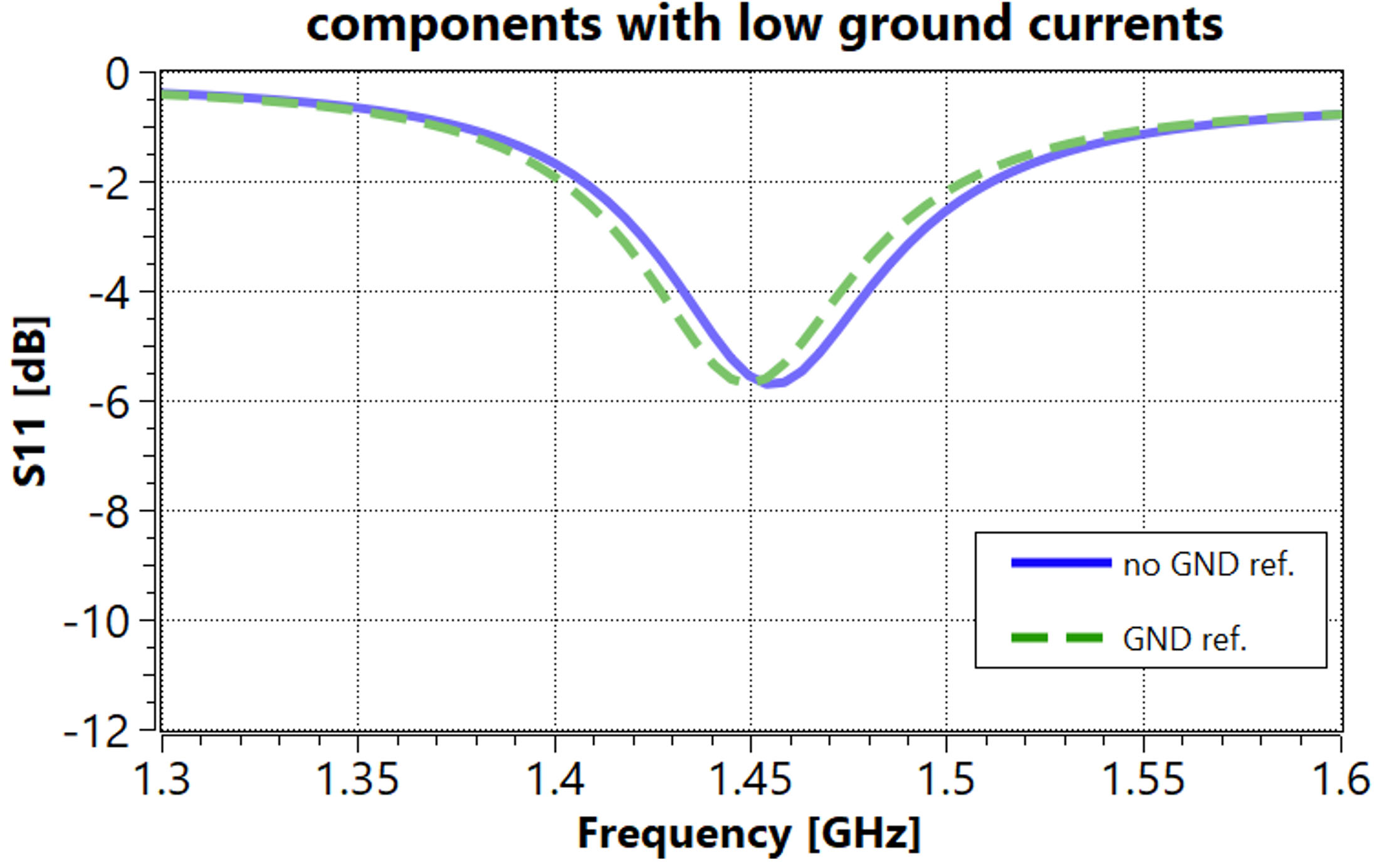
Figure 12. S11 at port 1 using a 5-port model (no GND reference), and a 9-port model (with GND reference), for the circuit with matching components with low ground currents.
The resulting picture is quite good – both methods (using component ports without ground reference and placing the component between two ground referenced ports) match using components with low coupling to the ground currents.
But let’s now check what happens if we use components with high coupling to the ground currents.
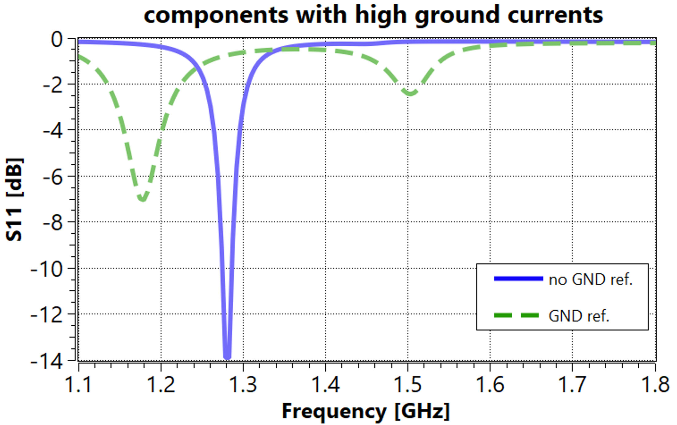
Figure 13. S11 at port 1 using a 5-port model (no GND reference), and a 9-port model (with GND reference), for the circuit with matching components with high ground currents.
There is a dramatic difference in results between methods with and without a ground reference for components with high ground currents.
Thus, the conclusion is more than clear.
When ground currents
are neglected, our
matching results go
haywire, especially
with components prone
to high ground
currents.
Conclusions
In conclusion, the impact of ground currents on antenna matching circuit optimization cannot be overstated. While simpler modeling approaches may seem appealing, they can lead us astray if not handled with caution. Here we discuss the pros and cons of two-port approach compared to the more popular single-port approach for lumped-element matching. However, this method requires duplicating the number of component ports used for matching, which can be computationally costly in terms of modelling time. A simpler EM model that uses only one port per matching component and does not reference the RF ground is attractive for simpler simulations of the targeted antenna designs. However, its use in circuit simulation treats the possible ground currents incorrectly. So, next time you’re fine-tuning your antenna matching circuit, remember to keep an eye on those sneaky ground currents – they might just be the key to unlocking optimal performance.
References
[1] S. Kosulnikov, M. Honkala, J. Rahola: ”The Role of Ground Currents in the Co-Simulation of Matching Components and Layout Models in Matching Circuit Optimization”, 18th European Conference on Antennas and Propagation (EuCAP 2024).
Field Application Engineer
sergei.kosulnikov (at) optenni.com