Power Balance Plots and Napoleon

Posted by Jussi Rahola | 18 December 2023

In this blog article, I will present the background and different variants of Optenni Lab’s power balance plots, which are used to illustrate power flow in RF circuits and antennas. But what has Napoleon to do with all this? Read through the blog and find out!

When delivering courses on matching circuit design at various conferences, I have used the following diagram to illustrate the power flow in matching circuits connected to antennas:

With this figure, it is easy to explain that the goal of matching circuit design is not to minimize the reflected power but to maximize the radiated power of the antenna system. The resistive losses of the matching components can indeed reduce the reflected power, but naturally this happens at the expense of radiated power and antenna efficiency.

Based on the above idea, back in 2019 we introduced power balance plots into Optenni Lab so that you can easily see the propagation of power in your antenna system and see the changes when you tune interactively any of the matching components. The figure below shows an example of the power balance plot for a single-antenna system, where also the absolute and relative power levels of the various loss mechanisms are shown numerically.

In addition to single-port matching, Optenni Lab can easily treat antenna systems with an arbitrary number of ports. The starting point is multiport antenna data coming typically from an electromagnetic (EM) simulator. Optenni Lab can synthesize matching circuits for each of the EM ports and wire the circuits to a number of external ports. In addition, Optenni Lab can optimize the type and value of components to be placed in the aperture or tuning ports of the EM model. The two figures below illustrate some possible multiport circuit synthesis setups in Optenni Lab.

Optenni Lab can easily plot the power propagation in multiantenna systems. The multiantenna  power balance plot can show the power lost to other ports (labeled “Coupling losses”) and depending on the setup the component losses can be in some cases shown for the feed port and for the other ports separately.

The animation below shows the power balance plot for the multiport antenna case when the user changes the visualization frequency.

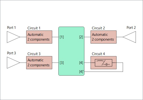
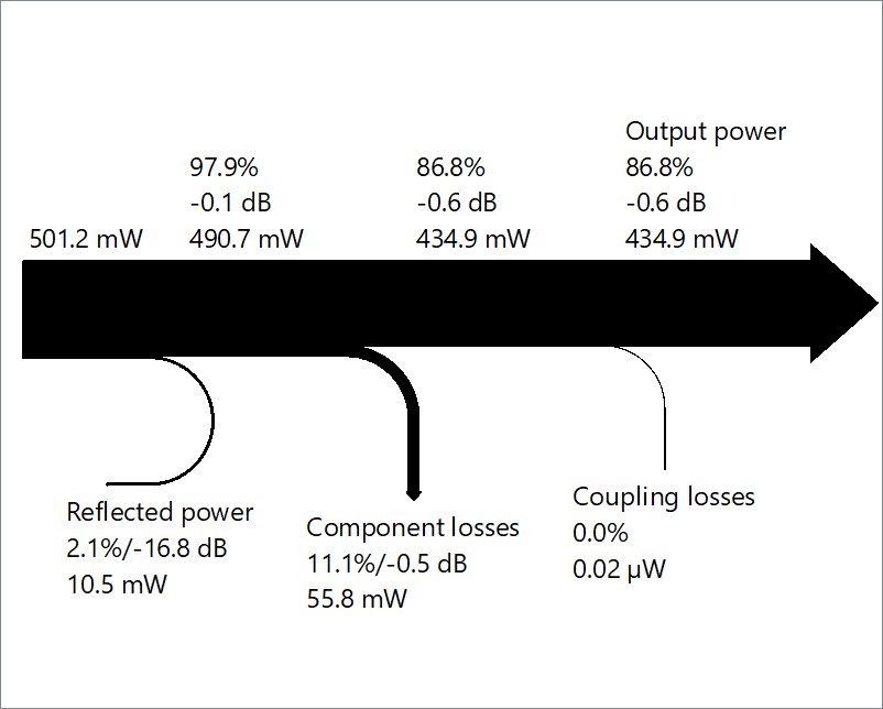
We also generalized the power balance plots to general RF systems, which do not have an antenna component. In this setup, Optenni Lab can easily show the power flow between a pair of external ports, where the goal is to maximize the power coupled to the target port (marked as “Output power”) and the power coupled to any other ports is considered as a loss (labeled “Coupling losses” in the image below).

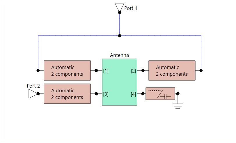
All the examples above assume that only one port is fed at a time. But Optenni Lab can also calculate the power balance plots for a simultaneous multiport excitation, such as in antenna arrays, where special emphasis needs to be placed on the active reflection coefficient and the dependence of the radiation efficiency on the feeding amplitudes and phases.

How does Napoleon then enter the picture? Well, during the IMS2023 exhibition I was demonstrating Optenni Lab and the power balance visualization to various customers and then two engineers independently remarked that the power balance plots resemble the visualization of the losses of Napoleon’s army during his infamous invasion to Russia during 1812.

Indeed, I studied Wikipedia and discovered the visualization by French engineer Charles Joseph Minard from 1869, which indeed uses related visualization techniques:

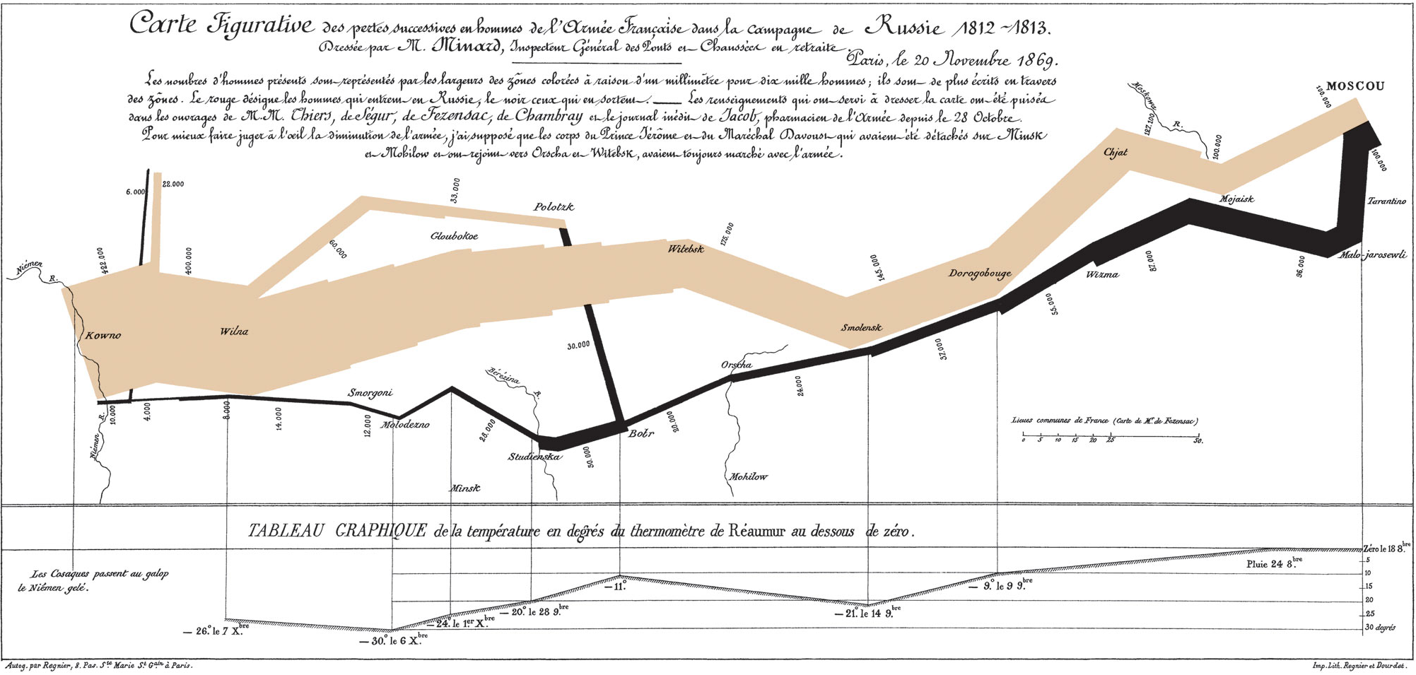
Source: Wikimedia commons.

From the visualization one can see the dramatic loss of life during this ill-fated campaign: over 400 000 solders started the march to Russia. Only some 100 000 reached Moscow and out of those only 4000 solders returned alive, others being eliminated by disease, exhaustion, and bitter cold. Quite a path loss!

In summary, we adopted a data visualization technique which is more than 150 years old to describe the power balance in antenna matching circuits and in general RF circuits. If your boss insists on focusing on the minimization of reflected power, you can use these plots to highlight the importance of maximizing the antenna efficiency instead.

CEO Jussi Rahola
Email: jussi.rahola (at) optenni.com